IBM® SPSS® Amos™ 28

This window allows you to pick any unknown data value and view its posterior distribution. To display this window, click on the toolbar in the Bayesian SEM window.

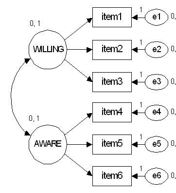
With the data and model of Example 32 in the User's Guide,

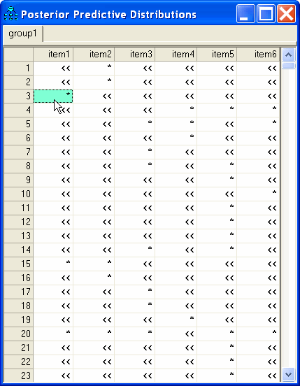
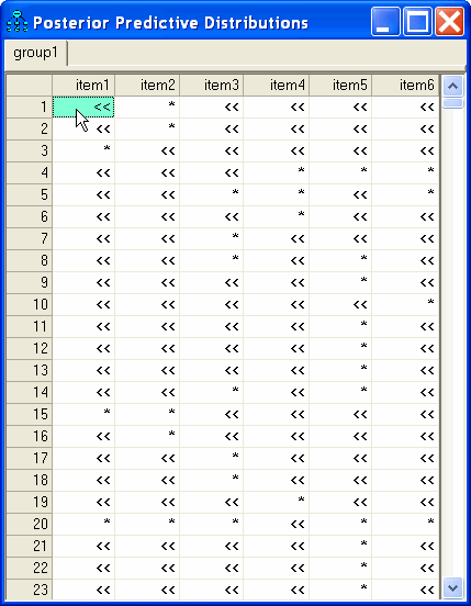
the Posterior Predictive Distributions window looks like this:

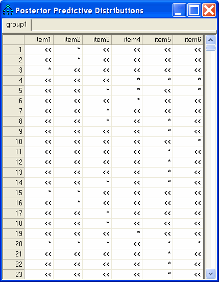
Each table entry in the window is one of the following.

▪A number in the case of an observed numeric value (There were no observed numeric values in this dataset.)

▪The symbol "*" for a missing value

▪The symbol "<<" for a data value that is subject to inequality constraints

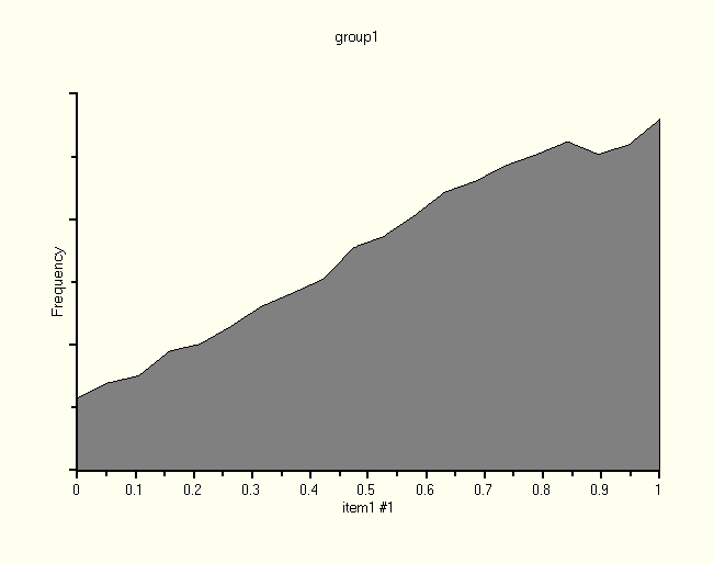
Clicking the table entry in the upper-left corner displays the posterior distribution of Subject 1's score on the numeric variable that underlies the response to item1.

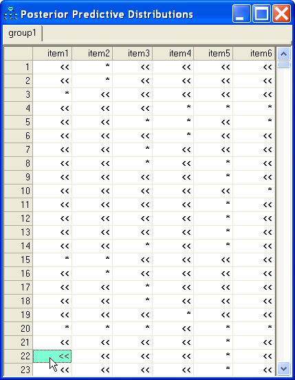
Clicking the entry in the 22-nd row of the first column displays the posterior distribution of Subject 22's score on the numeric variable that underlies the response to item1.

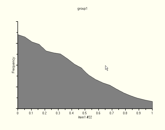
Notice that Subject 1 and Subject 22 gave the same response to item1, but our estimates of their scores on the underlying numeric variable are different.

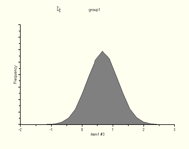
Clicking the "*" in the third row of the first column displays the posterior distribution of Subject 3's score on the numeric variable that underlies the response to item1.