IBM® SPSS® Amos™ 28

Menu: Analyze→D-Separation Preview

This window displays the result of a d-separation analysis.

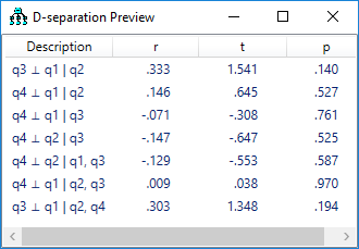
Here is the d-separation preview for Example 39 in the user's guide:

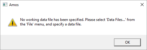
Looking at the first row of the table, the model implies that q3 and q1 are independent when q2 is "held constant". That is, q3 and q1 are independent in any subpopulation of people who share the same q2 score. This implies that the partial correlation between q3 and q1 with q2 "held constant" is zero in the population. The corresponding sample partial correlation is .333. The final two columns provide a test of the null hypothesis that the population partial correlation is zero, taking into account the facts that the sample partial correlation is .333 and that the sample size (N) is 22. 1.541 is a t statistic that has a t distribution with N - 3 = 19 degrees of freedom if the partial correlation is zero in the population (Weatherburn, 1968, page 256). The two-tailed "p value" is .140. That is, with a correct model the probability is .140 that a sample partial correlation would be as far from zero as it was in this sample. Each row of the table is interpreted similarly. None of the p values in the table is very close to zero, so that from this point of view the model in Example 39 is compatible with the data.You can get some d-separation results even without data. If you have the model of Example 39, but have not specified a data file, clicking Analyze→D-Separation Preview will display the  message

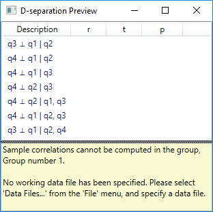
and then (after you click OK) the following list of d-separated pairs of variables.